
Show me the POCUS


Show me the POCUS
Physics
In this chapter we will review basic concepts to aid you in understanding the technology behind the clinical use of ultrasound and its limitations. These concepts will be used in the next chapters: Knobs and more, and Artifacts.
Showmethepocus.com contextualizes the concepts seen here:
Sound Waves
Sound waves are mechanical vibrations that induce alternate expansion (rarefaction) and compression of any physical medium (solid, liquid, or gas) through which the sound wave travels (with the exception of vacuum space). It is an oscillation of pressure transmitted through these mediums. These waves travel in a straight line and the medium's molecules move back and forth, or longitudinally. The particles do not travel all the way from the vibrating object (for example, from a speaker to the ear). A particle that is in resting condition is first disturbed causing it to vibrate which then exerts this force on the adjacent particle. That first particle then returns to its original position. The particles of the medium do not move forward themselves but the vibrations are carried forward and is visualized as a wave.
When particles move forward it compresses the air in front of it creating a region of high pressure and known as compression (C). When the vibrating object moves backwards, this creates a region of low pressure called rarefaction (R). The number of particles per given volume (density) has an effect on the pressure generated. Imagine shouting at sea level vs at Mt Everest were there is less pressure (not that this is advisable) but you would probably hear less because there are much less particles around you. The propagation of sound can thus be visualized as propagation of density variations or pressure variations in the medium.
λ

A
C
R
C
R
Density
or Pressure
Fig 1. Graphical representation of a sound wave. On the top, the sound wave as a sinosoid in graphic form representing how density and pressure change when a sound wave moves in the medium. A, amplitude; λ, wavelength. On the bottom the sound wave moving through the medium as a series of density and pressure variations as sound is generated from a speaker. C, compression and R, rarefaction. Image modified from Pluke in wikimedia.
We represent a soundwave graphically as a sinusoid waveform (Fig 1) with areas of compression representing the upper part of the waveform and maximum compression and density by the peak of the waveform. Rarefactions are represented by the lower part of the curve with low pression regions and the lowest pression and density region being the trough of the waveform.
Sound waves have four physical properties:
1. Amplitude (or loudness) is the height of the sound wave (A on the image above). As the sound wave increases in amplitude the medium will expand (rarefaction). Conversely, when the sound wave decreases in amplitude the medium will compress. Increasing the amplitude increases the acoustic pressure or the pressure generated by the sound waves. It allows the machine to hear a ‘louder’ return sound.
2. Wavelength ( λ ). The wavelength is the length of one wave cycle (i.e. from peak to peak) which includes one rarefaction and one compression.
3. Frequency. The frequency of a sound wave is the number of cycles of a sound wave per second given in Hertz (Hz). A small wavelength will yield a higher frequency. The human hearing range is 20-20,000 Hz while medical ultrasound is typically 1-20 MHz. Period is the time it takes for a single cycle to occur. Period is measured in time, wavelength is measured in length. A period is determined by the sound source, not the medium through which the ultrasound signal travels. Period and frequency are inversely related. A high frequency wave has a short period.
4. Propagation Velocity. Is the velocity that a sound wave travels in a medium. Propagation velocity is determined by the medium through which the ultrasound wave travels. Sound waves of the same frequency travel at different propagation velocities in different mediums. The propagation velocity of average human tissue is 1540 m/sec. That of air is 330m/sec and that of bone is 4080 m/sec. The propagation velocity is the product of wavelength and frequency. The wavelength can be calculated by dividing 1540 m/sec by the frequency. Note that wavelength is inversely proportional to frequency. A higher frequency will have a shorter wavelength. As the sound wave travels from one medium to another medium, the propagation velocity changes. This is important since the ultrasound machine assumes all tissues have the same velocities and the reason we appreciate artefacts (more on this later).
Transducers
The transducer is one of the most critical components of any diagnostic ultrasound system. There are many types of transducers and it is important to select the one appropriate for the planned application. Diagnostic transducers act as both transmitter and receiver of ultrasound. Beams generated can be directed to improve the quality of the image produced.
The primary component of the transducer is the piezoelectric crystal (see Fig 2.) composed of quartz or lead zirconate titanate. This crystal is the mechanism that allows transmission and reception of ultrasonic waves. It transmits ultrasound waves after being stimulated by alternating electrical current. These pulsed signals are reflected back to the piezoelectric crystal which then generates an electrical signal that is then processed and displayed.
The piezoelectric crystal is housed in a transducer which also contains a damping material, an acoustic lens and matching layer. When stimulated, the crystal vibrates in all directions with the majority coming from the front and back. This is inconvenient since we only need it do it from the front (the patient's side). The backing material (damping block) tries to eliminate vibrations on the back of the crystal and controls the length of vibrations from the front face. The matching layer improves (reduces) the acoustic impedance so that ultrasound waves can penetrate body tissue and allows the returning echoes to be return to the crystal for this same reason.

Fig 2. Cross section of an ultrasound transducer and its components. Image courtesy of Dr Rachael Nightingale, Radiopaedia.org, rID: 54040
The frequency of the transmitted ultrasound waves depends upon the type of crystal and its thickness. For maximal efficiency the crystal should be operating at its natural or resonant frequency and occurs when the thickness of the crystal corresponds to half its wavelength (λ/2). So crystal thickness is proportional to its wavelength and implies that a thicker crystal has a lower wavelength which will penetrate into tissues more than a thinner crystal. On the contrary thinner piezoelectric crystals produce higher electrical frequencies (lower wavelengths). To help you remember, thickness of the crystal should be proportional to the distance you are trying to scan.
The active crystals generate heat which can burn the patient and thus auto cool/auto shutdown safeguards are present.
Pulse length
A pulse of electricity is sent to the piezoelectric crystal and the crystal generates the ultrasound wave. The crystal is not stimulated during the next few milliseconds and it is during this time that waves that are reflected back to the transducer are received by the piezoelectric crystal and an electrical current is generated. The received signal can be processed and displayed. Short pulse length have an impact on the resolution of the image. A shorter pulse duration has better axial resolution than a longer pulse duration. Axial resolution is the ability to discern two separate objects that are longitudinally adjacent (one structure is slightly deeper than the other along the ultrasound beam).
Fig 3. Pulse length or duration and pulse repetition period. Image modified from echopedia.org.
Pulse repetition period.
Pulse repetition period is the time from the start of one pulse to the start of the next pulse. The transmission time and the listening time is the pulse repetition period. The length of a pulse can be changed by changing frequencies but the pulse repetition period is mainly determined by the listening time. The listening time is the time that the transducer can receive reflected signals from the transmitted beam. Once the depth of the ultrasound scan is increased, a longer listening time is required to be able to receive reflected signals. Therefore, the depth of the scan mainly determines the pulse repetition period. Pulse Repetition Frequency is inversely related to pulse repetition period. It is the number of pulses transmitted per second. A deeper scan requires a slower pulse repetition frequency to allow the deeper reflected signals to be received during the listening time
Depth of the structure
Assuming a constant speed and a fixed frequency the machine the location of each reflected ultrasound wave on the display. The image is formed by compiling these reflected scan lines. One image frame consists of many individual scan lines. The depth of a displayed image depends on the time delay between the transmitted and the returned signal. The ultrasound machine works on the presumption that soundwave is traveling at 1540 m/sec in blood. However if the tissue is able to slow the speed of sound the image displayed will appear to have a greater depth than what they appear on the screen.
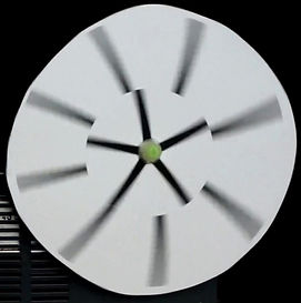
Aliasing
Aliasing is a measuring effect that causes signals to become indistinguishable from each other (Fig 4). Think of it as you are measuring the velocity of an object you cannot directly observe and have to sample at a certain rate. Picture throwing a ball into a wall. You sample the object with a camera taking only two pictures: when the ball close to the wall and when you are about to receive it. As far as your camera is concerned, the ball came from the wall. With aliasing your sampling rate of an object is such that the object is moving in the opposite direction. If the motion occurs faster than the maximal frame (sampling) rate, then the ultrasound machine is only intermittently capturing images or frames of the real motion.


01
02
Fig 4. Aliasing. On the left a stationary wheel with inner and outer spokes. On the right, the same wheel is moving in a clockwise fashion. It does so slow (01) and fast (02). The camera that captured these clips does so at 24 frames per second. If the speed of the spokes is more than the frames that the camera can capture then we have aliasing. The resulting effect is that instead of moving clockwise (01), we see the outer spokes moving anticlockwise (02). Clips modified from Pixelmaniac pictures.
In ultrasound machines many factors control the sampling rate. If the velocity of a measured object exceeds the sampling rate's capacity to display the maximum velocity, the wave's velocity is sampled opposite of it's true direction. Therefore, the wave is displayed as a velocity profile on the opposite side of the baseline. Since the velocity is exceeding the maximum velocity of the scale, it is displayed at the top of the opposite side of the baseline.
The Nyquist limit represents the maximum Doppler shift (explained below) that can be correctly measured without resulting in aliasing (color or pulsed wave ultrasound). The formula for Nyquist limit is:
Nyquist limit = Pulse Repetition Frequency /2
We can adjust the Nyquist limit on ultrasound machines to select low or high moving objects (Fig 5) . For high-velocity flow the PRF should be increased by adjusting to a higher Nyquist limit.
Lets take a look at some clips to use for reference:

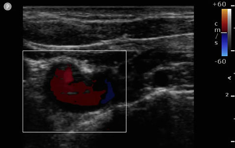
Fig 5.Adjusting Nyquist limit. In these clips we see a vessel being interrogated. The blood flow is physically going towards the probe and with Color Flow Doppler (explained below) this would represent on a red coloration of the vessel. On the left we have a low Nyquist limit and a high limit on the right. Aliasing is visibly occurring more in the left by having selected a lower Nyquist limit and thus a lower PRF. We thus see a mix of blue and red when in actuality it should be red. The arrows mark the Nyquist limit.
Probe Types
Transducers are described by their type and operating frequency that ranges from 2Mhz to 20Mhz. The different types of probes include phased array, linear and curvilinear.
The phased array probes are used when scanning deeper structures and the best one to scan the heart. The transducers are made up of individual elements that can each be independently driven and thus wave emission occurs at different phases. These ultrasound beams that are generated can be directed to improve the quality of the image produced. These probes are connected to specially-adapted drive units enabling independent, simultaneous emission and reception along each channel
Linear probes are used when interrogating shallow structures and can have either a small or wide footprint. Curved linear proves are used for deeper structures such as when interrogating the abdomen and have a wide footprint.
Fig 6. Probe Types: Phased array (surface and transesophageal), linear and curved linear.
Interactions with Tissue
As the ultrasound beam penetrates a medium, the beam loses energy in what is known as attenuation. As a beam is transmitted and penetrates tissue, some of the beam is reflected, refracted or absorbed as heat generation. The amount of penetration will determine the depth of the scanning area. Penetration is directly related to wavelength. Smaller wavelengths are more easily reflected or refracted in the superficial tissues than longer wavelengths. A larger wavelength will penetrate deeper. This is why you select probes with lower frequencies to penetrate to deeper tissues.
Even the most advanced ultrasound machines there are interaction with tissues. This interaction is responsible for measurement errors, artifacts, and poor picture quality. It is important to understand to avoiding errors and misdiagnosis.
Ultrasound waves interact with tissue in four basic manners. Those interactions are:
1. Reflection
Reflection occurs when the ultrasound wave is deflected back towards the transducer. The major factors affecting the amount of reflection are:
i. Angle of incidence is the angle of the ultrasound beam and the tissue plane. It occurs at tissue boundaries and tissue interface. Tissue boundaries that are perpendicular to the ultrasound wave's path act as excellent reflectors and if the reflector is smooth and the wave strikes at 90 degrees then the reflection is strong and called specular. Those tissue boundaries that are parallel to the ultrasound wave's path act as poor reflectors. As you can imagine when the ultrasound wave is not reflected the ultrasound signal is not recorded and the display shows a lack of signal or dropout of the ultrasound picture. Tissue boundaries that are smooth and have a width greater than the ultrasound wave act as a mirror or a specular reflector which results in a significant amount of reflection of the signal.
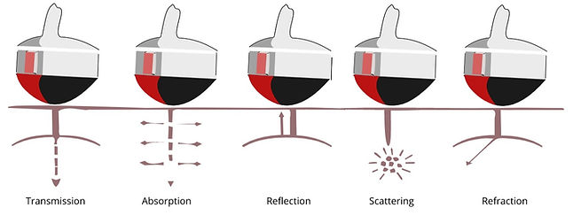
Fig 8. Angle of incidence. B mode apical 4 chamber view. Notice that the resolution of the mitral valve and that of the posterior atrium (white arrow) is better than that of the interatrial septum (red arrow). In fact you may notice there is drop out (loss of signal) and it appears as though there is a patent foramen oval when it may or may not exist.
ii. Acoustic impedance. Acoustic impedance is the ease with which sound wave propagates through a medium and is determined by the density and stiffness of the tissue. Think of it as the resistance to ultrasound transmission. When the ultrasound wave travels through one medium into another a change in acoustic impedance occurs. This amount of change will determine the amount of reflection and thus what you see on the US screen. Large changes in density between two tissues will result in a large change of acoustic impedance. The difference in acoustic impedance between two tissues accounts for the amount of reflection that will occur at the tissue border. This is why cannot interrogate deep lung tissue well with ultrasound since the majority of the ultrasound waves are reflected at the plane between the pleura and the lung.

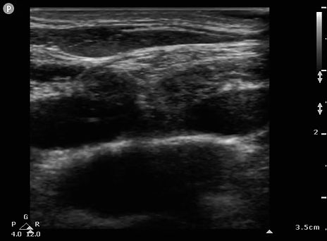
Fig 9. Acoustic impedance. On these clips we are visualizing the same supraclavicular structures. On the left, the probe was used without the use of ultrasound gel. On the right, with gel. The absence of gel makes for a high acoustic impedance and thus we start with limited ultrasound transmission. Notice the area of absence of echoes denoted by the arrows because of the high impedance.
2. Refraction.
Refraction is reflection where sound strikes the boundary of two tissues at an oblique angle. The reflections generated do not return directly back to the transducer. Refraction occurs when the ultrasound signal is deflected from a straight path and the angle of deflection is away from the transducer. Refraction only occurs at a different medium interface of different acoustic impedance. If the propagation velocity is greater in the first medium, refraction occurs towards the center or converges. If the velocity is greater in the second medium, refraction occurs away from the originating beam or diverges.

Fig 10. Side lobe artifact as an example of refraction. Side lobes reflect sound from a strong reflector outside of the central beam. Echoes are displayed as though they originated from the central beam and thus appear in the center of the display. This transverse US of the urinary bladder displays this kind of artefact. There is only urine in the urinary bladder even though the reflectors have caused side lobe artifacts making it appear as though there is actually something there.
3. Attenuation
Attenuation is the reduction in amplitude of the ultrasound beam as a function of distance through the imaging medium. As the ultrasound wave travels through a medium, the medium absorbs some of the energy of the ultrasound wave. The amount of energy absorption, or acoustic impedance (Z), is determined by the product of the density of the medium and the propagation velocity of the ultrasound wave. During attenuation the ultrasound wave stays on the same path and is not deflected. As it passes through tissues of different densities, the amplitude decreases. Once all of the ultrasound wave energy is absorbed then structures distal to the point of total attenuation will not be visualized and will appear to be dropped. Attenuation is frequency dependent. Low frequencies have better penetration and are therefore not attenuated as much as higher frequencies.
Fig 11. Shadowing as an attenuation artifact. Shadowing is caused by partial or total absorption of the sound energy that prevents us to see structures that are deeper. In this example we see rib shadowing and makes it hard for us to see the liver and kidney.
4. Absorption.
At each plane of ultrasound beam penetration some of the ultrasound waves are absorbed by the tissues and produce heat.
Energy is lost by reflection, scattering, and attenuation. The loss in energy results in a "noisy" background on your monitor. If the signal-to-noise ratio is good then a clear picture will be displayed. A poor signal-to-noise ratio results in a blurry picture. We can counteract the loss of signal during the assessment of deeper structures by altering the power (energy emitted) or gain/TGC (amplification of the returning signals).
Resolution
Resolution is the ability to distinguish between two points in space (location with regards to each other) and temporal (location with regards to time).
Spatial resolution of an ultrasound beam is defined in three planes: axial, lateral, and elevational planes. Axial resolution is the ability to discern between two points along or parallel to the beam's path. Lateral (Alzmuthal) resolution is the ability to discern between two points perpendicular to a beam's path.
Axial Resolution
Axial resolution is dependent upon: Wavelength and pulse length. A higher frequency wavelength can differentiate two structures more easily than a longer wavelength. The general rule is that if the distance between two points is less than one wavelength these will be displayed as one structure. If on the other hand this distance is more than the wavelength then two structures will be displayed. A shorter pulse length will discern two structures more easily than a longer pulse length. Measurements taking along the beam's path rather than laterally are more precise because the axial resolution is typically better than lateral resolution.
The formula for axial resolution is as follows:
Axial resolution= 1/2 x SPL
SPL is the spatial pulse length and corresponds to the number of cycles generated and the wavelength of a pulse. The lower the SPL, the lower the axial resolution which is what we want. A lower axial resolution implies better axial resolution.
Lateral Resolution
Lateral resolution, or the ability to discern between two points in the lateral plane and depends on beam width and frequency. It is the ability to discern between two points perpendicular to the beam path. A small wavelength will discern two points more easily than a larger wavelength. A narrow beam width can discern two points better than a wide beam. Beam width is the most important factor in lateral resolution.
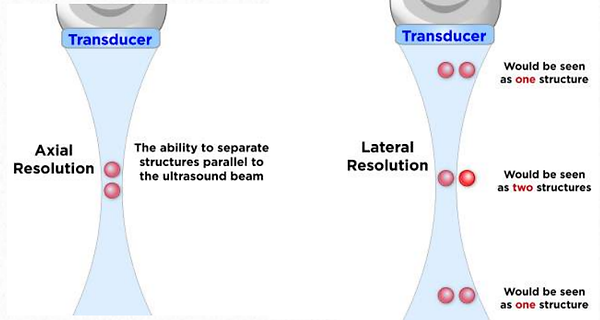
Fig 12. Axial vs Lateral resolution. Image courtesy of Foresight Ultrasound.
Temporal Resolution is the resolution that tracks moving targets over time and as you can imagine it is worse with higher depths as it takes longer to return, large scanning sector or high line density and higher pulse repetition period (or low pulse repetition frequency) because it takes longer to send a pulse and receive it.
Resolution and penetration are inversely related. At the high penetration/low resolution settings the deeper structures are more easily visualized at the loss of resolution of more superficial structures. In a high resolution/low penetration setting the deep structures are not well visualized while the superficial structures have improved visualization.
Optimizing Your Ultrasound Image
The following methods can help you maximize the image resolution so that you can get the best temporal and spatial resolution (this will be explored further on the next section):
1. Using the lowest depth possible to visualize the structure of interest. This selects the highest possible frequencies and thus the best resolution possible. Also note that the pulse repetition frequency is lower since the probe has to 'listen' for longer periods of time on the returning signals that are further away. The pulse repetition period is longer in deeper structures for the same reason. In short, a deeper structure has worse resolution, a high pulse repetition period and a low pulse repetition frequency.
2. Selecting the appropriate focus depth of your machine. This appears with a marker on the right hand side of your screen. You can change its location by going more shallow or deeper. The focus feature should be selected to the area of interest you are trying to interrogate.
3. Gain and Time Gain Compensation (TGC) are both post-processing adjustments that attempt at amplifying the returning signals. Overall the image brightness is adjusted so that all tissues appear either brighter or darker since it does not affect the resolution of tissues. TGC allows us to selectively adjust the depth location (or path length differences) that we want gain to be either increased or decreased. These are 'bands' of gain that can be adjusted.
4. Increasing the Power: This relates to the strength of the voltage spike applied to the crystal for each pulse. Increasing power output increases the amplitude of the beam or the 'loudness' and therefore the strength of echo returned to the transducer. This feature increases heat.
Ultrasound Modes
01 Brightness or B MODE
This is the standard method for image creation in 2 dimensions. The returning echoes are displayed on a television monitor as shades of gray. This represents a 2 dimensional image of approximately 3mm in depth. Typically, the brighter gray shades represent echoes with greater intensity levels. The best image is created when the object of interest is orthogonal. The image is displayed with grayscale brightness corresponding to the intensity of returning signals.
The brightness displayed on the screen is determined by the amplitude (loudness) of returning echoes: Anechoic is complete or near absence of returning sound waves and represented black. Hypoechoic has very few echoes and is represented darker than surrounding tissues. Hyperechoic signals are high amplitude and represented whiter than surrounding structures.
We could stop here and not go any further for focused POCUS exams since this is all that we need for them. However ultrasound has many more features that are explored further.

Fig 13. B mode. Short axis view of the heart on B mode. Here the ventricular walls appear isoechoic and pericardium hyperchoic.
02. M-Mode (or Movement Mode)
A single scan line is interrogating the space. The image displayed is the behavior of those structures of interest on that scan line and time. This mode provides the greatest temporal resolution and so it is very useful for moving structures particularly if they are moving fast.


B mode. Short axis view of the heart on B mode.
Fig 14. M mode scan of the short axis of LV. Notice the scan line in the middle of the scan sector. As soon as you turn on that scan line will receive echoes from on that particular line and generate an image of the movement of that structure (y axis) over time (x axis) and create the image on the right. Notice here that we can accurately measure distances and the displacement of structures. In this example we can correlate the EKG with the mechanical movement of motion of the heart. The QRS on the EKG and start of systole occur in close proximity with one another (red line with arrows)
The other modes we will mention rely on the Doppler effect and so we take a pause and revisit that effect here:
03 Color Doppler:
Color Doppler uses the Doppler effect to color code changes in frequency. The Doppler shift occurs when the emitting and receiving frequency are different. Returning echoes from positive or negative doppler shifts (toward or away from the transducer) are displayed with corresponding colors to indicate direction of flow. The color doppler window can be adjusted and represents a window of pulsed wave doppler signals that has been assigned a color representation for its direction and velocity of flow.
The range of the velocities that you are measured with Color Flow Doppler is shown on a legend on the screen. This range of velocities is called the Nyquist limit and corresponds to the maximum amount of velocity measured. By changing this range you can make a small patent foramen oval appear or disappear from the screen so it is important to have this set up to an adequate range. For fast moving flow such as valves, use 60cm/s as a good reference. When the velocities of the structure of interest are greater than the measuring velocities we have aliasing.
The Doppler effect
Lets take a look at the Doppler effect closely. The Doppler effect is the measured change in frequency that corresponds to a change in velocity which in turn is related to a change in flow. Lets dig a bit deeper for better understanding.
The ultrasound probe emits a frequency that travels to a vessel. This vessel contains moving red blood cells that interacts and reflect this sound wave. The reflected sound wave then returns towards the probe with a different frequency to that which was emitted. If the red blood cell is moving away from the probe, its wavelength is higher and has a lower frequency.
Let imagine we have an ambulance with a siren emitting the same frequency. If the vehicle remains stationary we perceive one unique frequency but if we hear and ambulance coming towards us and then moving away from us we hear a difference in frequency due to the movement of the vehicle. If its coming towards us the frequency appears higher since the wavelengths are compressed together. Once the ambulance moves away from us the wavelengths now are further and further away from each other and we perceive a lower frequency. The faster the moving object, the greater the perceived change in frequency. We can also display this information visually which is what the US machine would do for us. If this Doppler effect of an object moving away from us we would be displaying it blue and red if the contrary were true which is what happens when you turn on the Color Flow Doppler (CFD) feature of the machine.
1
2
Fig 15. Schematic representation of the Doppler effect with the use of a an ambulance and a active siren. On the left, a human ear representing the ultrasound sensor. 1, stationary ambulance. 2, moving ambulance
This Doppler shift is thus directly proportional to the speed of moving red blood cells and ultrasound machine creates a spectral display of the different changes in velocity observed. It is important to note that to be able to measure this shift in frequency we need to be as parallel as we can to the flow and that at 90 degrees from flow we are unable to detect any doppler shift. An important feature of Pulsed Wave Doppler (see below) which is a technology that uses Doppler is that we can measure this shift in a particular point in space with the use of a gate.
This doppler change represents flow velocity with the following mathematical formula:
This math formula is important since it describes the velocity as being directly proportional to the Doppler shift. Of the parameters, C is the speed of sound in the medium and corresponds to 1541m/s in soft tissue. Ft is the frequency of the probe and in order to penetrate to deeper tissues we need a lower frequency and thus this parameter does not change much. Theta (θ) is the angle between the emitted wave and the direction of flow. The larger this angle, the worse the error in measurement.
Doppler Shift x C
Flow velocity =
2 x Ft x Cos θ
Fig 16. Color Flow Doppler turned on while interrogating the right subclavian artery. The probe footprint is on the supraclavicular fossa and aimed at the heart. Blood should be flowing towards the probe and why we see a red hue on the subclavian artery on this clip.
Other doppler modes examine the characteristics of direction and speed of tissue motion and blood flow and present in spectral displays as well as sound:
Pulsed Wave Doppler (PWD)
Pulsed wave Doppler uses the Doppler effect but only on a very small window on single scan line (see the image below). It thus measures changes in velocity on a specific structure along the scan line. It is ideal to measure left ventricle outflow track when assessing patients for fluid responsive. The insonating angle should be as close to 0 as possible meaning that the flow on the structure of interest should be as parallel the insonating beam. In the example below we are interrogating the flow on that particular gate on the middle cerebral artery on PWD and we can appreciate flow (velocity in cm/s) on the y axis, against time. This allows us to generate a quantitative analysis of flow on that particular gate.

At
Vd
Vs
Fig 17. Example of spectral Doppler frequency display of the middle cerebral artery. B-mode US with Color Flow Doppler sector overlaid. PWD sample box over the middle cerebral artery. Peak systolic velocity (Vs), end systolic velocity (Vd), acceleration time or systolic upstroke (At), pulsatility index (PI), time-averaged mean maximum velocity (Vmean) (traced in purple).
Continuous Wave Doppler
The Doppler effect is also used here. This time however all the velocities coming from that scan line (and not a particular point in that scan line) is measured. So you measure all velocities that are coming towards the probe which means you can measure high velocities but you cannot tell where they are coming from (something called range ambiguity). This is a great technique for measuring the highest velocity across a narrow path such as that which can occur in patients with aortic stenosis.

A
B
Fig 18. Example of spectral Doppler frequency display of the Left ventricular outflow tract (LVOT). In these images we are attempting to interrogate the aortic valve. Images taken from the apical 5 chamber view. B-mode US with Color Flow Doppler sector overlaid. We are thus obtaining transvalvular pressure gradients and assume that the narrowest point is at the level of aortic valve (untrue if a patient has hypertrophic cardiomyopathy). In image A we appreciate CWD and the spectral doppler window it generates over all velocities across that scan line. In B, the PWD sample box is over the LVOT. A CWD with a maximal velocity of more than 4m/s is indicative of aortic stenosis. In this example it is 4.8m/s. We can also compare the PWD to CWD ratio spectral profile with the velocity time integral (VTI). VTI is the calculated are over the curve and it represents velocity across time. Another indicator of aortic stenosis is the VTI of the LVOT / VTI of the Aortic Valve and a value less than 0.25 is considered severe aortic stenosis. Image from Santangelo G et al.
Bioeffects
Ultrasound has thermal, cavitation, and other effects on tissues. The thermal effects of ultrasound causes the temperature of tissue to increase. Dense tissue such as bone is less likely to disperse the energy of an ultrasound wave and temperature rises faster. Blood on the other hand disperses the heat very easily.
As the ultrasound intensity (power) or frequency increases the rate of rise of the temperature increases. Activating color modes greatly increases the power of the ultrasound output. In 2D mode the temperature will rise slower than in color mode. When the ultrasound is not in use, the probe should be disconnected or placed in "freeze" mode so no power is transmitted to the probe tip. The temperature of the probe should not exceed 10 degrees centigrade of the patient's temperature or a burn injury can occur.